Part 1 of 5 in the LibriBrain series. The project page summarises the whole project.
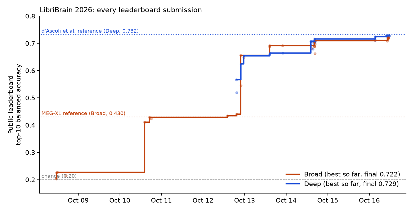
The LibriBrain 2026 competition asks which of fifty words a listener heard, given 306 channels of magnetoencephalography (MEG) recorded while they listened. A prediction counts if the true word is among its ten best guesses, scored as balanced accuracy over the fifty words, so chance is 0.20. The Deep track has one listener with about eighty hours of recordings; the Broad track has thirty-nine others, most with ten to forty minutes of labelled data and seven with none. My entry scored 0.722 on Broad and 0.729 on Deep on the public leaderboard, against published references of 0.430 and 0.732, on a single 8 GB GPU. On the final private leaderboard (2 November 2026) it scored 0.678 on Broad, 17th of 53, and 0.697 on Deep, 26th of 91.
The target matters more than the network
Each word is represented by a three-second window of MEG around its onset, clipped to its own sentence. A convolutional encoder turns the window into an embedding, and a four-layer transformer lets the words of a sentence inform one another. The change that mattered was the training target. Rather than only classifying among fifty labels, the model learns to predict, for every heard word, the contextual embedding a large text model (T5) assigns to that word in its sentence, using all of the roughly one million words in the training audio. That single change took the Broad score from 0.23 to 0.43. Depth, width, window length and training time each moved it by a point or two.
One deep reference brain
The second jump was unexpected. A model trained on the Deep listener alone, then applied to the Broad listeners with no adaptation, scored 0.66. Adding the Broad listeners’ own recordings to training made transfer steadily worse, from 0.632 locally with none of their data to 0.452 when it made up half of each batch. Ten to forty minutes from a new head appears to add more variation in sensor geometry and noise than information about words, while eighty hours of one brain gives a clean mapping that generalises.
Structure inside each listener’s own data
The test set has structure that each listener’s own unlabelled rows reveal, and three steps exploit it without ever combining data across listeners.
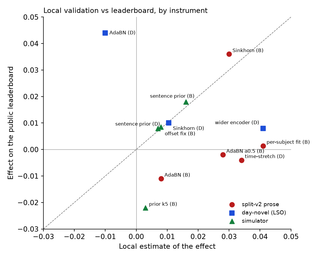
- Class balancing. The model inherits the skew of ordinary prose, where the is far more common than people. Rescaling each listener’s predictions so every word receives equal total probability added 0.036 on Broad.
- A self-learned grammar. Each listener heard 156 sentences built only from the fifty words. A small bigram model fitted to that listener’s own decoded sentences, with no text corpus, added 0.018 on Broad.
- Recording-day correction. The Deep test set came from a day absent from training. Re-estimating the network’s normalisation statistics on those recordings added 0.044 on Deep.
The timing-only baseline
All listeners heard the same sentences, and the test files exposed enough timing to align rows across people. That alignment was prohibited, and the entry never used it. There is a subtler version of the same problem inside each sentence. The spacing between words encodes their durations, and durations identify short function words well.
To measure it, I trained a classifier with no brain data at all, using only what each test row exposes: the word’s position, the gap to the next word and the sentence length. On the same held-out blocks where the brain decoder scores 0.70 to 0.78, the timing-only model scores 0.632. Duration alone gives 0.468. This gives a strong non-neural baseline on the tested split. Comparing a decoder with timing-only prediction is necessary to assess how much performance depends on the neural measurements. My entry uses no timing features.
Validation that tracks the leaderboard
Local validation needs care on data like this. Held-out quarters of the same recording sessions overstated several changes that later added nothing on the leaderboard, because a model can learn something specific to a session that the test set does not share. Two instruments tracked the leaderboard well: a model trained with an entire recording day held out, and a simulator built from real held-out predictions arranged into sentences shaped like the test set. The simulator reproduced the grammar’s leaderboard gain almost exactly (+0.016 against +0.018) and let me screen more than 160 post-processing ideas in the final two days.
Where the evidence runs out
If a listener’s predictions are averaged over repeated hearings of the same word, grouped using the true labels, accuracy rises by 0.14 with four hearings and 0.22 with sixteen. The information exists in aggregate. Without labels, however, those repeats cannot be found: in every raw representation tested, two trials of the same word are no more alike than two different words. The binding constraint is the evidence a single hearing leaves in the sensors, and the next real gains will come from the measurement itself: more repetitions per word, sensors closer to the scalp, or better source models.
The code, the pre-registered experiment log and the development history are at github.com/rohit-ravi2/libribrain-2026.
Next in the series: Building my LibriBrain speech decoder, the story of how these ideas came together.