Part of the ANN–BNN series. Project page: Where an inference law lives.
In October I spent a week looking for a quantity that artificial and biological learners would share at the level of the synapse: a write cost per bit, measured in weights for one and in plasticity for the other. Eighteen operationalisations failed or were true by construction. The failure was not bad luck. It was a category error about where the shared thing lives, and the point of this series is the correction.
Three components
Any learner, animal or network, is three coupled things.
| component | what it is | in an animal | in a network |
|---|---|---|---|
| prior | the inductive bias each episode starts from | innate circuitry, shaped by development | architecture plus pretrained weights |
| inference | the state update given data, inside an episode | persistent activity, neuromodulatory state, short-term plasticity | the forward pass; attention over context |
| write | the transfer from state to durable structure | synaptic plasticity, consolidation | a gradient step on weights; absent at deployment |
The October arc looked for an invariant in the third row. The laws that actually held were in the second.
Why the similarity is close, and why it carries so little
The laws I was chasing come from animal conditioning. Trials to acquisition fall as a power of (C/T − 1), where C/T is the ratio of the background cycle between rewards to the cue duration; Harris and Gallistel (2026, eLife) fit a slope of −0.66 across 14 rat groups at a 4:1 odds criterion, regressed on log(C/T − 1). Rescaling every interval by the same constant changes nothing: the law is timescale invariant. A truly random pairing of cue and reward produces no learning (Rescorla, 1967).
None of these is a fact about neurons. Estimating a rate from sparse, delayed events is a Poisson problem, and the Poisson problem is scale free: multiply all times by a constant and the posterior over the ratio of rates is unchanged. The C/T slope is how evidence accumulates for an ideal observer, whose log likelihood ratio per reinforcement is log(C/T) minus a gap term. Any learner that approaches the normative solution inherits both properties. A meta-trained transformer is one trained across many episodes drawn from a distribution of tasks, so that its forward pass over the context of a new episode does the episode’s learning; for uniform-attention transformers that in-context predictor is provably close to the Bayes-optimal one on the training distribution (Wakayama and Suzuki, 2025). So a transformer meta-trained on such streams should reproduce the laws with no biological ingredient at all, and the one I trained did: acquisition in context, no acquisition on a shuffled control, and no effect of T at fixed C/T (medians of 5, 5 and 6 trials at T of 4, 12 and 36 for C/T 4.5; 3, 3 and 3 for C/T 27).
That reproduction is the null expectation, not the discovery. When a law is a theorem of the task, finding it in two systems says they both solve the task; it says almost nothing about how. I made a related argument about perception in an essay on certainty: a sign that is present just as fully when a hypothesis is wrong as when it is right adds no evidence of its own. A shared law is that kind of sign for a shared mechanism.
Where the difference can live
If inference is where the laws are, the differences between the two kinds of learner have to be in the other two rows.
The prior’s provenance. In Gallistel’s account, rats do not learn the C/T law; they arrive with it. For a transformer the prior is whatever the meta-training distribution installed, so it is exactly as wide as that distribution. The prediction that follows is about edges: a network’s prior should fail at the boundary of its training range, an animal’s at the boundary of its ecological range, and the shape of the failure, not the in-range slope, is the substrate signature. My C. elegans work is a caution about how much a wiring diagram fixes of a prior: the multimodal pipeline treats the worm’s genome-specified wiring as a given, and on its own later tests found that the wiring alone did not predict recorded activity, which is itself a statement about how little a connectome fixes. The anatomy explorer for the biophysical model inventories what such a substrate represents explicitly, channel by channel and synapse by synapse; that inventory is the prior and the machinery of inference, not the write.
The write channel. Biology has a continuum of plasticity timescales, and state-level inferences are consolidated into structure selectively, gated by a few broadcast neuromodulators. A deployed network has no write at all: whatever it inferred in context is gone at the end of the episode. A training network has a write of enormous bandwidth with no gating by what was inferred in state. The two are limited in opposite directions, and that is the row where a comparison can be informative.
The inference-only signature
The cleanest single prediction from the decomposition is a split inside the spacing effect. Trials to acquisition as a function of C/T is an inference-level fact, and in-context learning reproduces it. Retention after spaced versus massed training is, in this decomposition, assigned to the write. A learner with no write channel should therefore show the acquisition law and no retention structure: no forgetting, and no advantage of spaced over massed training at long delays.
I wrote that prediction down, hashed it (sha256 prefix 229d51ac050c0bee), and scored it on the meta-trained transformer. Same streams as before, T = 12, massed at C/T 4.5 and spaced at C/T 27, eight reinforcements, then a single probe cue at a delay D of 0.5, 2, 8 or 32 cycles after the eighth. The readout is the paired belief at the probe: the model’s predicted wait on the contingent stream against the same model’s prediction on the control stream, scaled so that the acquisition asymptote is 1. Twenty seeds.
| C/T | belief at last acquisition cue | D = 0.5C | D = 2C | D = 8C | D = 32C | hierarchical Bayes (all D) | fixed-parameter Bayes, D = 32C |
|---|---|---|---|---|---|---|---|
| 4.5, massed | 1.21 | 1.23 | 1.40 | 2.03 | 2.87 | 1.00 | 0.03 |
| 27, spaced | 1.06 | 1.05 | 1.09 | 1.21 | 1.42 | 1.00 | 1.00 |
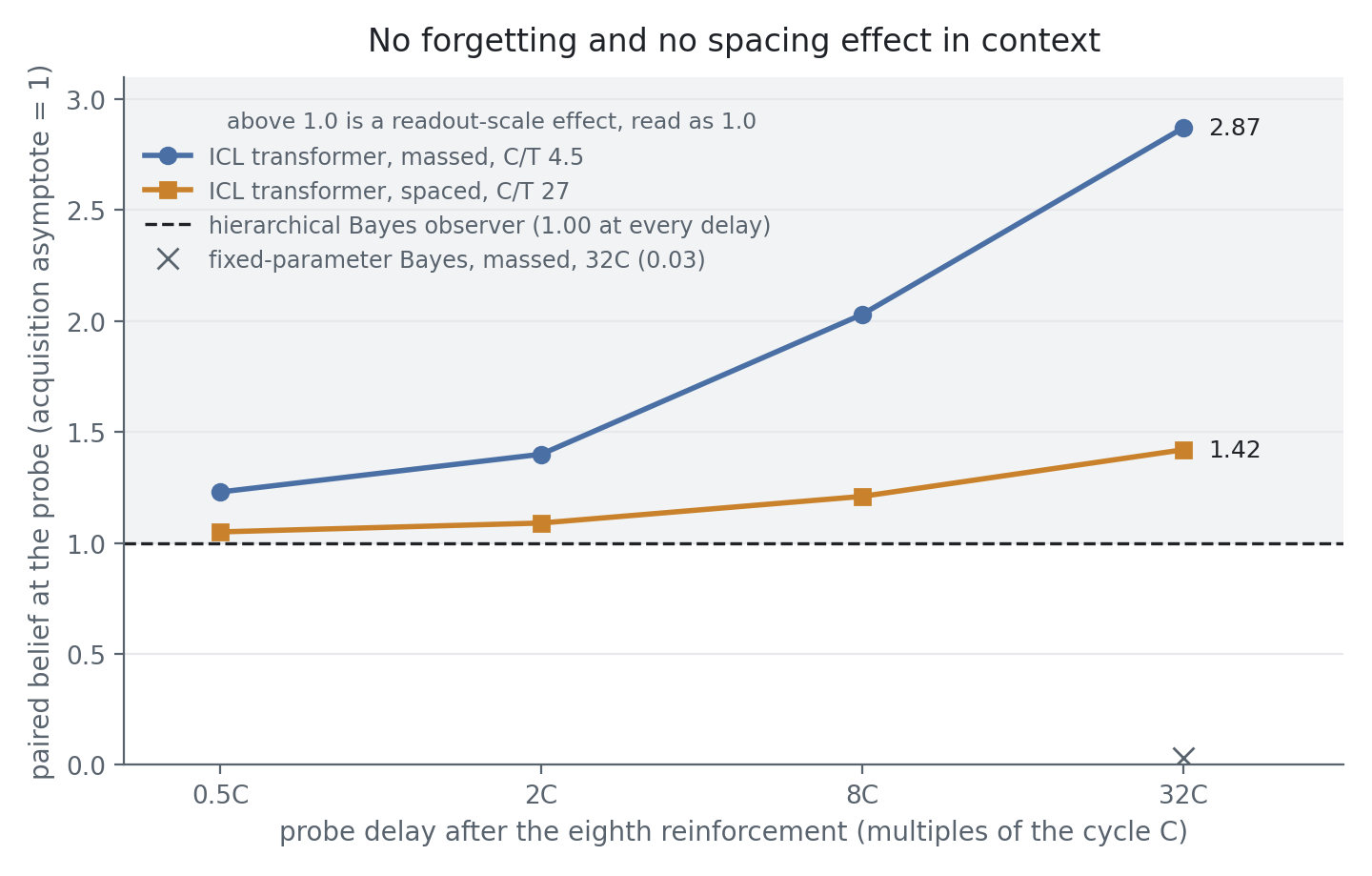
First, the pre-registered verdict, because it is not the one the table invites. The predictions file fixed the reference as a Bayes observer that treats C and T as known, and asked that the model track it within 0.2 at every delay and show a spaced-minus-massed difference below 0.2. On that reference and the raw readout, P1 fails: the first clause fails in 6 of 8 cells (massed 0.24, 0.41, 1.07 and 2.84 from the reference; spaced 0.05, 0.09, 0.21 and 0.42), and the spacing clause fails at 8C and 32C, where massed exceeds spaced by 0.82 and 1.45, the opposite of the animal direction. Two things I did after seeing the results turn that into the flat profile I describe next: a hierarchical reference, written after the result files, and a rule that clips the readout to 1. Both are defensible, and both are post hoc, so the flat profile is reported as exploratory and not as a pre-registered pass.
With that label on: no retention decrement at any delay, for either spacing. The fraction of seeds with belief at or above 0.8 is 0.90 to 1.00 in every cell of the primary checkpoint, and a second checkpoint trained with an even prior over contingency lands within 0.15 of every value at or below 8C and 0.25 apart at the 32C massed probe, both above the readout ceiling. Values above 1 are a scale artefact of the paired readout (at long gaps the control stream’s predicted wait grows while the contingent prediction stays near T) and are read as 1.0. There is no spaced-over-massed advantage, and no massed-over-spaced one once the scale artefact is removed. That is the inference-only signature the decomposition predicted for an instrument with no write.
Two things in the table are worth more than the headline. The reference had to be fixed before the result meant anything. A Bayes observer that treats C and T as known collapses to 0.03 at the 32C massed probe, because a gap that long is nearly impossible under contingency with those parameters. An observer that marginalises C and T over the meta-training prior (a 60 by 40 grid) holds 1.00 at every delay: the long gap is explained by “C is larger than I assumed”, not by “the contingency is gone”. The transformer agrees with the second observer. Before a departure from the ideal can be charged to the substrate, the ideal has to carry the same prior family as the learner, and the honest record is that I learned this from the result, not before it. Second, the extinction arm of the same probe is uninformative about inference and informative about the prior. Training streams were stationary, so eight reinforced trials followed by forty unreinforced ones has probability zero under both training hypotheses. The low-prior checkpoint drifts to extinction in a median of about 20 trials massed, counting the 2 of 20 seeds that never extinguished within 40 as censored (18 if they are excluded), and 12 spaced with none censored; the checkpoint trained with an even prior never extinguishes within forty trials (20 of 20 censored). Out of distribution, the prior decides, which is a provenance signature and not a law.
The other half
The I-only signature is half of a dissociation. The other half is a learner with a write channel showing the animal pattern on the same streams, and that is the week of hashed runs in the next post. I will say here what the first of them established about substrate, because it belongs to this argument. A leaky GRU with the same meta-training, weights frozen, forgets in absolute time: at the 32C probe its belief is 0.16 on the massed schedule and 0.00 on the spaced one, while the hierarchical observer holds 1.0. Its timescale invariance breaks once the cycle exceeds the state time constant: at C/T 27, T = 36 needs 13 trials against 4 at T = 4. It also breaks, unexplained, at the short end, where at C/T 4.5 with T = 4 it needs 14 trials against 3.5 at T = 12; that one is not a leak signature and is recorded, not interpreted. Neither break is a law of the task. The first is a signature of a state that leaks, which is to say a fact about the inference carrier, found exactly where the decomposition says substrate should show.
Nothing in this post is a claim about brains. It is a claim about where a comparison between learners can be informative, and the first measurement on the row where it cannot.